Regression Discontinuity Design
Review of RDD
RD is based on the seemingly paradoxical idea that rigid rules create valuable experiments.
There are two distinct features of RDD. When \(a\) is our running variable, first, treatment status is deterministic of \(a\) and second, Treatment status is a discontinuous function of \(a\).
There are two types of RDD: First, Sharp RDD - Treatment cleanly switches on or off once running variable passes threshold. Second, Fuzzy RDD - Probability or intensity of treatment jumps at a cutoff.
Summary of Meyersson (2014)
Islamic Rule and the Empowerment of the Poor and Pious
Several countries have experienced Islamic political parties coming to power through democratic elections. This paper examines whether democratically elected Islamic polticians lead to worsened women’s rights.
This study implements RDD to answer this question using data from Turkey. Short answer is No! Islamic rule increases female secular high school education.
Turkey was founded as a secular republic but the influence of Islam in politics has increased substantially over the years. Secular education was viewed as a fundamental step toward modernization. Secular education includes mixed-sex education and banning of wearing religious symbols in school e.g. headscarf for women
In 1994, the pro-Islamic Refah Party became the second largest party in terms of votes. This brought about an unprecendented representation of Islamic political party and education facilities tailored to religious conservatives
Challenge in Identification
Comparing between municipalities with an Islamic or secular mayor is not sufficient since assignment of mayor type is non-random. For example, municipalities more likely to elect an Islamic mayor may have some unobserved characteristics that also influence female enrollment.
RDD can help. Assignment of treatment (i.e. mayor type) is determined solely on the basis of a cutoff score on an observed running variable (i.e. win margin for the Islamic party relative to the largest non-Islamic party). In a narrow range, treatment is assigned almost randomly.
Methodology
This study combines 1994 election data and 2000 census data at municipality level. Using RDD, it compares education outcomes where an Islamic mayor barely won or lost the election.
\[ y_i = \alpha + \beta m_i + f(x_i)+\epsilon_i, \] where \(m_i = 1\{x_i\geq c\}\).
It also conducts RD validity checks: whether density of running variable is continuous at discontinuity and whether control variables jump at the cutoff.
Results & Discussion
Having an Islamic mayor increases female enrollment by 3 percentage points. Effects for men are smaller and imprecise. This result contradicts a commonly-held belief that religious state leads to worsened women’s rights.
In religiously conservative communities, the headscarf ban, mixed-sex classes, and a secular curriculum create barriers to enroll in school for religious women. Islamic parties overcome these barriers by allowing headscarfs and creating facilities more amenable to religious conservatives.
Replication
Download replication data
Visit https://erikmeyersson.com/research/ \(\rightarrow\) Publications \(\rightarrow\) “Islamic Rule and the Empowerment of the Poor and Pious” \(\rightarrow\) STATA replication files and load regdata0.dta to R working environment.
library(haven) #import dta data
library(tidyverse)
data <- read_dta("regdata0.dta") %>%
  select(hischshr1520f, hischshr1520m,
         i94, vi1, vshr_islam1994, partycount, lpop1994,
         ageshr19, ageshr60, sexr, shhs,
         merkezi, merkezp,buyuk,subbuyuk,
         starts_with("pd_")) %>%
         na.omit() #2629 observations
Variable explanation
- hischshr1520f : Share women age 15-20 with high school education
- hischshr1520m : Share men age 15-20 with high school education
- i94 : Islamic mayor in 1994
- vi1 : Islamic win margin
- vshr_islam1994 : Islamic wote share 1994
- partycount : Number of parties receiving votes 1994
- lpop1994 : Log population 1994
- ageshr19 : Population share below 19 in 1994
- ageshr60 : Population share above 19 in 1994
- sexr : Gender ratio in 2000
- shhs : Household size in 2000
- merkezi : District center dummy
- merkezp : Province center dummy
- buyuk : Metropolitan center dummy
- subbuyuk : Sub-metro center dummy
OLS specifications
ols <- lm(data = data,
          hischshr1520f~vi1)
coefficients(summary(ols))[,1:3]
## Estimate Std. Error t value
## (Intercept) 0.15302526 0.003015656 50.743599
## vi1 -0.03565611 0.008426467 -4.231442Estimation with OLS yields negative estimates, meaning that globally, Islamic rule lowers female high school enrollment.
However, note that mayor type is not exogenously determined. We can improve this using RDD.
RD Validity Checks
First check whether there is positive density around cutoff.
hist(data$vi1, 100, main = "Histogram of Islamic win margin",
     probability = TRUE)
abline(v=0, col = "blue")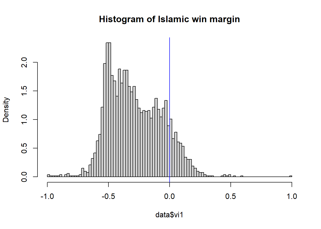
Next, check whether there is a jump in control variables.
library(rdrobust)
rdplot(data$vshr_islam1994, data$vi1,
       ci = 95, # confidence interval
       nbins = c(40,40), #number of dots on each side
       binselect = "es", #bins are evenly spaced
       x.lim = c(-0.25, 0.25),
       y.label = "Islamic vote share",
       x.label = "Islamic win margin")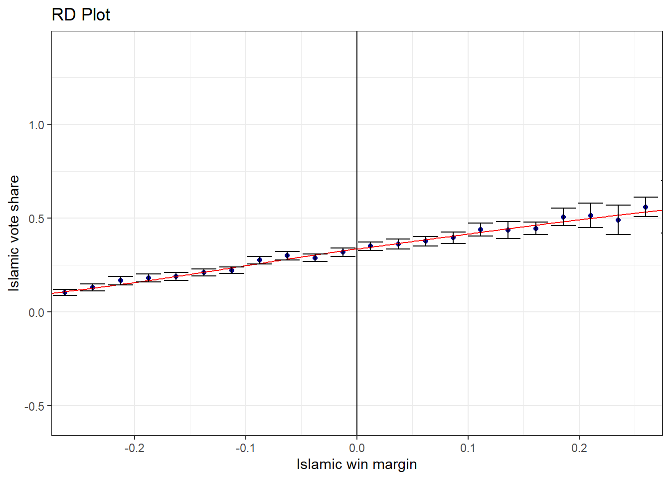
Repeat the exercise for all covariates.
control <- list(data$vshr_islam1994, data$ageshr19,
                data$sexr, data$partycount,
                data$ageshr60, data$lpop1994,
                data$merkezi, data$shhs)
varname <- c("Islamic vote share","Age 19-","Gender",
             "Number of parties","Age 16+","Log population",
             "District Center","Household size")

for (i in 1:length(control)) {
  rdplot(control[[i]], data$vi1,
         ci = 95, # confidence interval
         nbins = c(40,40), #number of dots on each side
         binselect = "es", #bins are evenly spaced
         x.lim = c(-0.25, 0.25),
         y.label = varname[i], x.label = "Islamic win margin")
}
Graphical Illustration of RDD
rdplot(data$hischshr1520f, data$vi1,
       ci = 95,nbins = c(20,20),binselect = "es",
       y.lim = c(0,0.25),x.lim = c(-0.5, 0.5),
       y.label = "Share of 15-20 year-old women with high school degree",
       x.label = "Islamic win margin")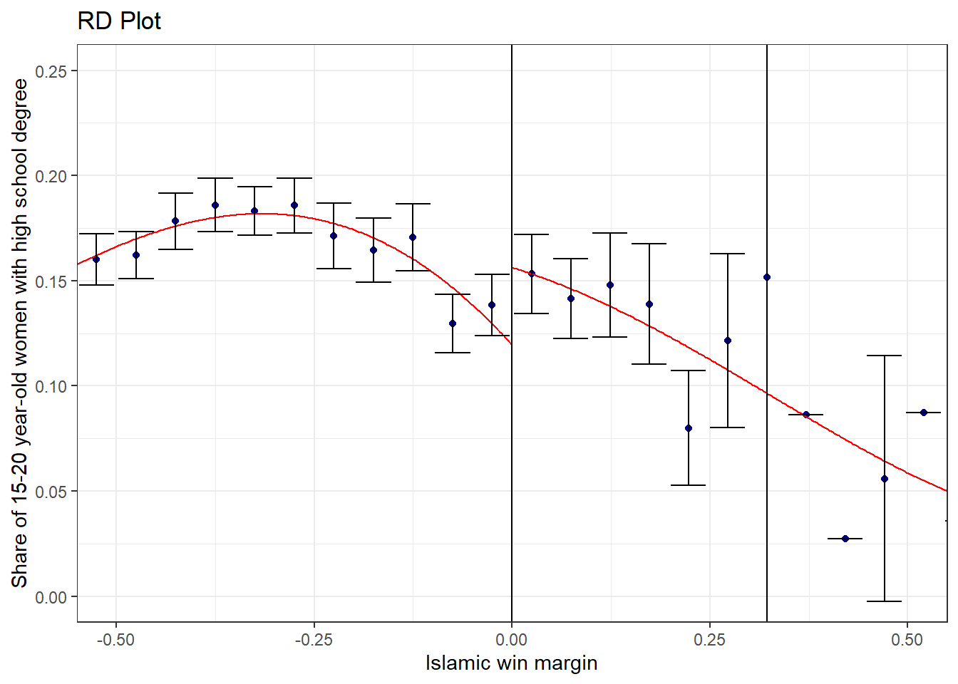
rdplot(data$hischshr1520m, data$vi1, ci = 95,nbins = c(20,20),
       binselect = "es", y.lim = c(0,0.25),x.lim = c(-0.5, 0.5),
       y.label = "Share of 15-20 year-old men with high school degree",
       x.label = "Islamic win margin")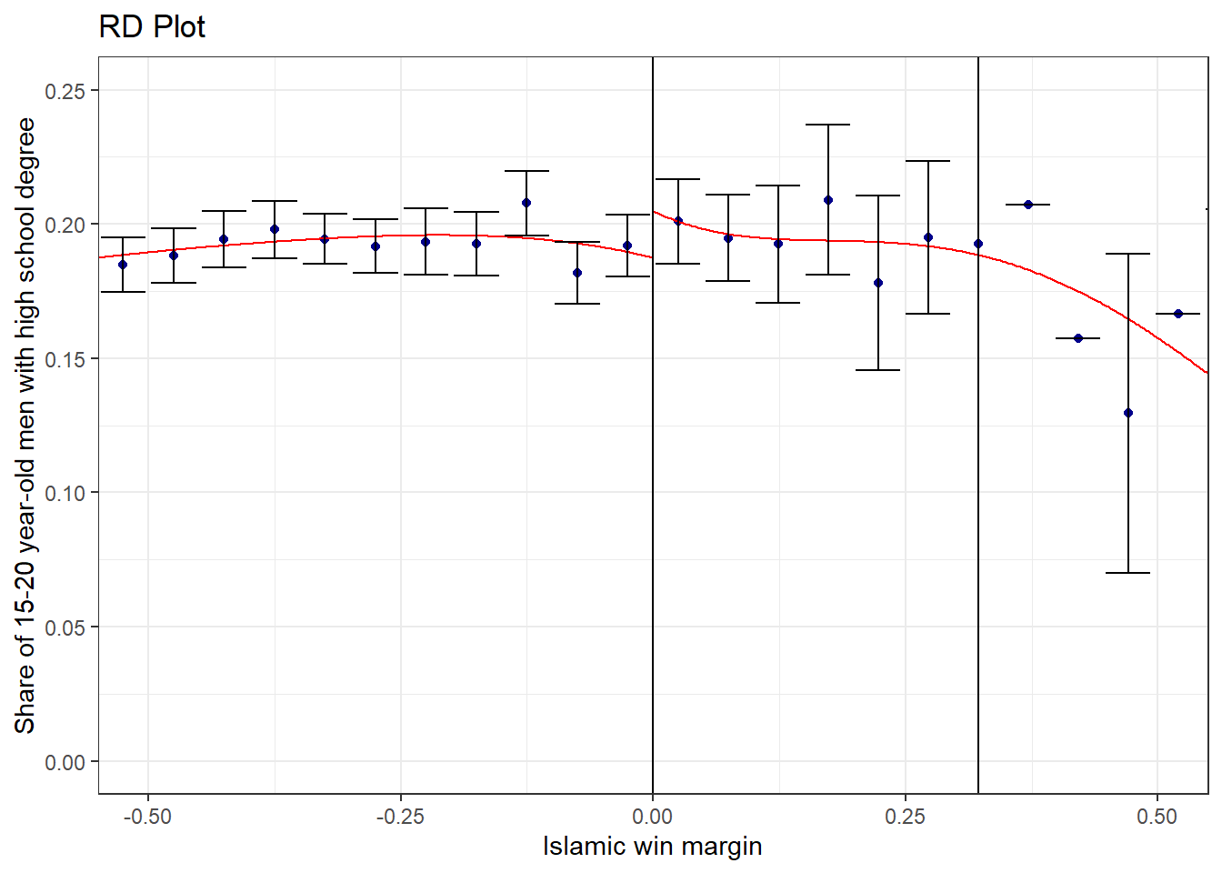
Bandwith selection
We need to choose how many observations to include in the regression. Optimal bandwidth used in this study is the one calculated from Imbens and Kalyanaraman (2012) algorithm.
library(rdd)
band <- IKbandwidth(data$vi1, data$hischshr1520f)
band
## [1] 0.2397612RDD Estimation without Covariates
rd_est <- RDestimate(hischshr1520f~vi1,cutpoint=0,bw=band, data=data)
summary(rd_est)
##
## Call:
## RDestimate(formula = hischshr1520f ~ vi1, data = data, cutpoint = 0,
## bw = band)
##
## Type:
## sharp
##
## Estimates:
## Bandwidth Observations Estimate Std. Error z value Pr(>|z|)
## LATE 0.2398 1020 0.02963 0.01241 2.388 0.01696 *
## Half-BW 0.1199 589 0.02502 0.01647 1.519 0.12869
## Double-BW 0.4795 2049 0.02279 0.01009 2.258 0.02397 *
## ---
## Signif. codes: 0 '***' 0.001 '**' 0.01 '*' 0.05 '.' 0.1 ' ' 1
##
## F-statistics:
## F Num. DoF Denom. DoF p
## LATE 4.988 3 1016 3.876e-03
## Half-BW 1.704 3 585 3.303e-01
## Double-BW 25.744 3 2045 4.441e-16LATE corresponds to the estimation with optimal bandwidth. 1020 observations are used.
Half-BW (Double-BW) is when narrower (wider) bandwidth is used, resulting in fewer (more) observations.
An Islamic mayor leads to approximately 3 percentage points increase in women’s highschool enrollment. The effect is statistically significant.
What we just estimated is Sharp RDD. For Fuzzy RDD, see the documentation of ?RDestimate.
Next, consider RD estimate for males. Don’t forget to obtain a new optimal bandwidth.
##
## Call:
## RDestimate(formula = hischshr1520m ~ vi1, data = data, cutpoint = 0,
##     bw = band_m)
##
## Type:
## sharp
##
## Estimates:
##            Bandwidth  Observations  Estimate  Std. Error  z value  Pr(>|z|)
## LATE       0.3230     1342          0.011561  0.009089    1.272    0.2034
## Half-BW    0.1615      747          0.019136  0.011913    1.606    0.1082
## Double-BW  0.6460     2584          0.008664  0.007469    1.160    0.2460
## ---
## Signif. codes:  0 '***' 0.001 '**' 0.01 '*' 0.05 '.' 0.1 ' ' 1
##
## F-statistics:
##            F       Num. DoF  Denom. DoF  p
## LATE       0.8750  3         1338        0.9068
## Half-BW    1.4627  3          743        0.4469
## Double-BW  0.9692  3         2580        0.8126
The effect is not statistically significant. This means Islamic rule has significant positive impact only on female education attainment.
Plotting RDD estimates
plot(rd_est, range=c(-0.6,0.6))
abline(v=0) 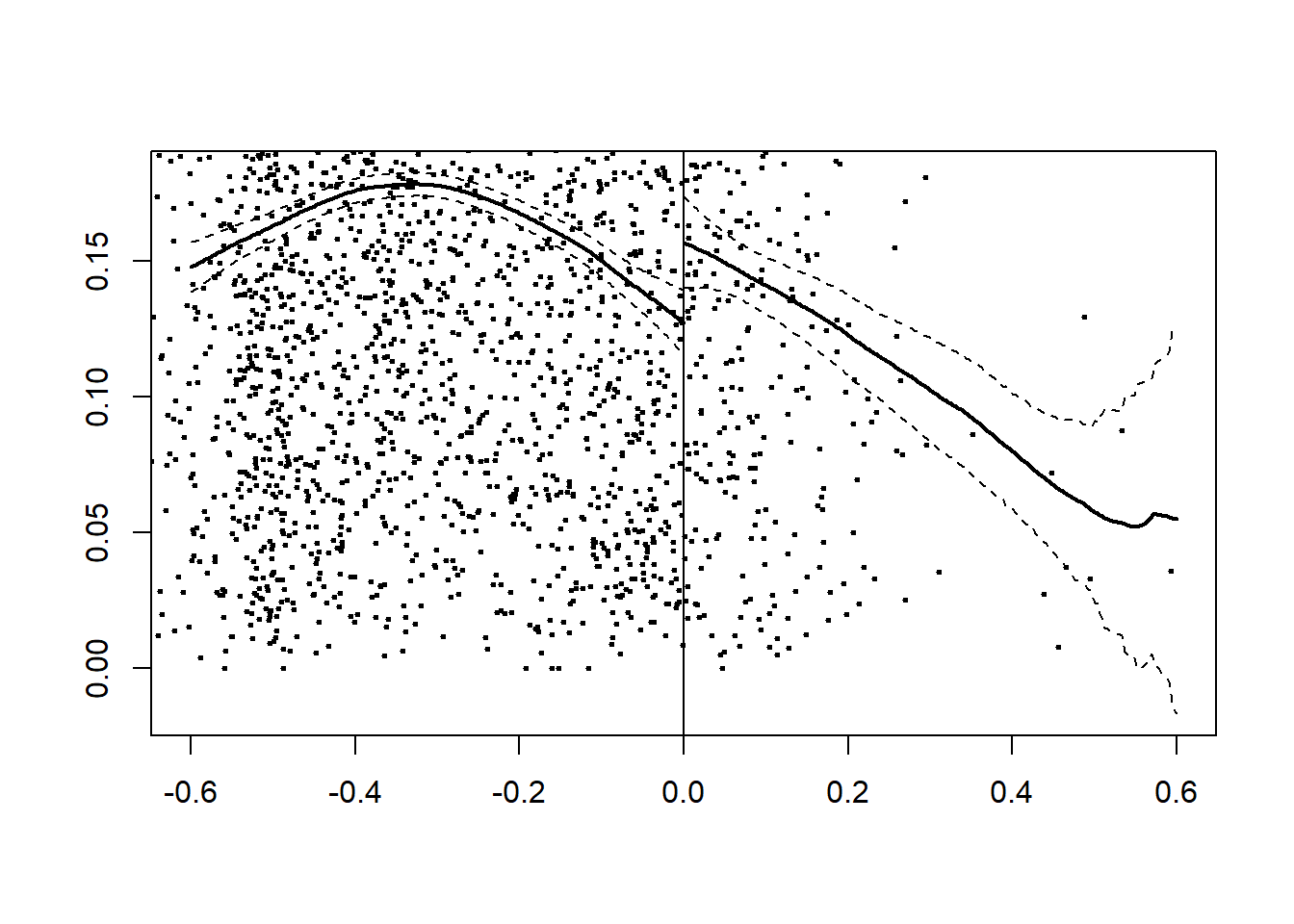
plot(rd_estm, range=c(-0.6,0.6))
abline(v=0) 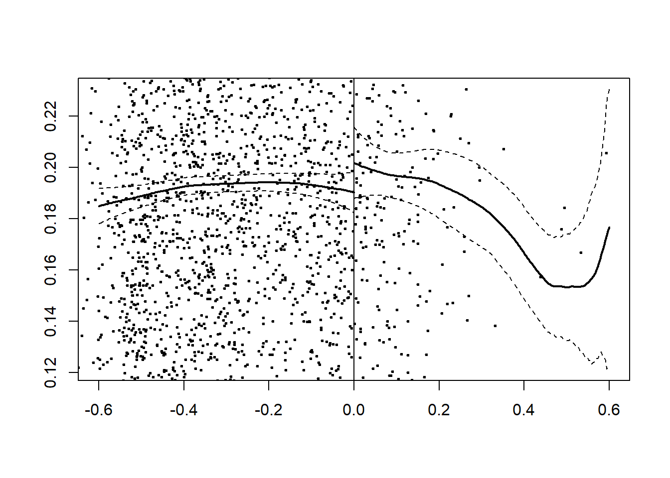
RDD Estimation with Covariates
provinceFE <- data %>%
  select(starts_with("pd")) %>%
  select(-pd_1) %>%
  as.matrix()

rd_est_control <- RDestimate(hischshr1520f~vi1 |
                       vshr_islam1994 + partycount +
                       ageshr19 + ageshr60 + sexr + lpop1994 +
                       merkezi + merkezp + buyuk + subbuyuk +
                       provinceFE,
                     cutpoint=0,
bw=band, data=data)summary(rd_est_control)##
## Call:
## RDestimate(formula = hischshr1520f ~ vi1 | vshr_islam1994 + partycount +
## ageshr19 + ageshr60 + sexr + lpop1994 + merkezi + merkezp +
## buyuk + subbuyuk + provinceFE, data = data, cutpoint = 0,
## bw = band)
##
## Type:
## sharp
##
## Estimates:
## Bandwidth Observations Estimate Std. Error z value Pr(>|z|)
## LATE 0.2398 1020 0.02563 0.007843 3.267 0.0010853
## Half-BW 0.1199 589 0.02891 0.010793 2.679 0.0073932
## Double-BW 0.4795 2049 0.02334 0.006441 3.624 0.0002901
##
## LATE **
## Half-BW **
## Double-BW ***
## ---
## Signif. codes: 0 '***' 0.001 '**' 0.01 '*' 0.05 '.' 0.1 ' ' 1
##
## F-statistics:
## F Num. DoF Denom. DoF p
## LATE 18.13 92 927 0
## Half-BW 11.35 88 500 0
## Double-BW 32.57 93 1955 0